Research Application Technology Center, Park Systems Corp.

Introduction

  Atomic force microscopy (AFM) is a powerful tool that can be used to obtain information on surface morphology of target materials in correlation with their frictional, electrical, mechanical, and thermal properties at the nano-scale. In particular, Lateral force microscopy (LFM) is an AFM technique that allows studying of the frictional properties quantitatively. Using LFM, friction information can be collected at various operational and experimental conditions (e.g., applied force, velocity, temperature, humidity, and vacuum). Hence, LFM can provide a big picture on the overall frictional behavior of material and be helpful in design and selection of material to meet the requirements for specific applications. For example, LFM has been used for studying of frictional and tribological properties of two-dimensional (2D) materials (e.g., graphene, MoS₂, and h-BN) which are potential candidates as protective and solid lubrication coating layers for micro- and nano- devices [1,2]. However, LFM measurement is not always straightforward due to lack of guideline on experimental procedure and data interpretation. Especially, quantitative measurement of frictional properties can sometimes be cumbersome for a new AFM user. This study aims at providing a helpful approach on how to measure the quantitative frictional properties at the nano-scale using the AFM.

How LFM works

  The principle of LFM is similar to that of Contact mode AFM. In Contact mode, the vertical bending of cantilever is monitored while AFM tip scans on surface to collect information on surface morphology of the sample. In LFM, twist of the cantilever is additionally monitored to collect information on distribution of frictional properties across the sample surface. Fig. 1 presents schematic illustration of a typical LFM measurement. Essentially, the Z scanner will press the tip against the sample surface until a given vertical deflection setpoint, as denoted in Fig. 1(a). This setpoint force will be kept constant during scanning. To collect the LFM data, the tip should scan on the sample surface in a direction perpendicular to the cantilever axis (∆X). The lateral (friction) force exerted at tip-sample interface will generate a torque τ that twists the cantilever about its axis, causing the displacement in lateral direction of the laser spot on the quadrant position sensitive photo detector (PSPD), as shown in forward scan and backward scan illustrations in Fig. 1(a). By monitoring the lateral signal while scanning forward and backward on the sample surface, a friction loop data can be generated, as shown in Fig. 1(b). The friction force acted between tip and sample is half width in vertical direction of the friction loop.

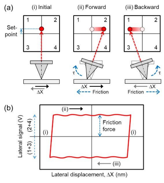
Fig. 1. Illustration of a typical LFM measurement. In LFM, the laser spot displacement in vertical direction [(1 + 2) – (3 + 4)] and lateral direction [(2 + 4) – (1 + 3)] are monitored to provide information on surface topography and frictional properties of target sample. In (a), the cantilever behavior during scanning is shown. Friction-induced torque τ will twist the cantilever about its axis, leading to lateral displacement of the laser spot on PSPD. In (b), an example of friction loop obtained from LFM measurement is shown. The half width of lateral signal is defined as friction force in unit of volts.

Example of LFM measurement

  A Park NX10 AFM system was used in this study. To obtain a clear LFM signal, a cantilever with relatively low spring constant is preferred to enhance the lateral force sensitivity. In this regard, a conventional Si probe (PPP-CONTSCR, Nanosensors) with nominal spring constant of about 0.2 N/m was used for measurement. Prior to data collection, the cantilever was calibrated in both normal and lateral directions for quantitative normal and lateral force measurements, respectively. Fig. 2 presents a typical normal force calibration procedure in AFM. The normal deflection sensitivity or A – B sensitivity (in volts per micrometer) of the cantilever was determined by performing force-distance (FD) curve measurement on a rigid substrate (e.g., silicon or sapphire substrate). Generally, the A – B sensitivity can be calculated from linear portion of forward or backward curve using the integrated function of SmartScan AFM control software. However, as shown in the data Fig. 2(a), the A – B sensitivity determined from backward curve was found to be slightly larger than that of forward curve due to effect of sliding friction between the AFM tip and the sample in this work [3]. To eliminate this effect, the A – B sensitivity was calculated by taking average of values determined from forward and backward curves. As a result, A – B sensitivity was calculated to be 29.04 V/µm. Then, thermal noise method [4] was used to determine the normal spring constant of the cantilever. For a more representative result, about 200 thermal spectra were collected and averaged. The spring constant of the cantilever used was calculated to be 0.21 N/m, from the fitting result in Fig. 2(b).

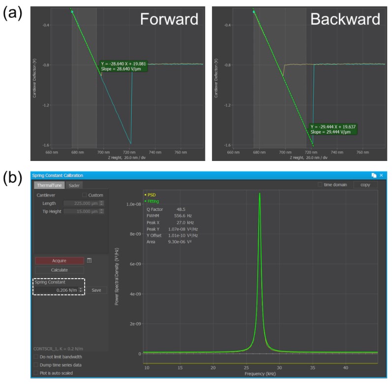
Fig. 2. Example of normal force calibration in AFM. In (a) the A – B sensitivity of the cantilever was determined from the force-distance curve. In (b), the embedded thermal tune function can be used to calculate the spring constant of cantilever based on thermal noise method.

  Lateral AFM Thermal-Sader method [5–7] was used to determine the lateral force sensitivity of the cantilever. This method has advantages of simplicity, tip preservation, and good accuracy [5–7]. Thermal noise spectrum of the first torsional vibration mode of the cantilever was collected. A signal access module was used to connect LFM signal from the PSPD to A – B input of the controller, as shown in Fig. 3. Examples of normal and torsional vibration modes of the same cantilever are also presented in the figure. The first normal and torsional resonances were found to be at about 27 kHz and 278 kHz, respectively, for the cantilever used. Then, the first torsional mode of the cantilever was fitted to the simple harmonic oscillator (SHO) model to determine the dc power response Pdc, torsional resonance frequency fT, and quality factor QT based on Eq. (1).   where PSD(f) is power spectral density as a function of frequency f, Pwhite is noise floor of thermal signal. Fig. 4 shows an example of the SHO model fit to the first torsional mode of the cantilever with Pwhite, Pdc, fT, and QT as fit parameters. For lateral force sensitivity calculation based on Lateral AFM Thermal-Sader method, Pdc, fT, and QT are required.

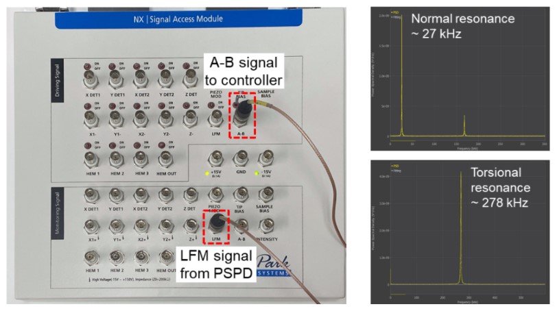
Fig. 3. Experimental set-up for lateral calibration. The signal access module was used to direct the LFM signal from the PSPD to A – B input of the controller to collect the thermal noise spectrum of the first torsional vibration mode of the cantilever. Noted that the switch at A – B port can be turned off to collect normal thermal signal as usual and turned on to collect lateral thermal signal.

  In the next step, torsional Sader method [8] was used to calculate the torsional spring constant kT of the cantilever. For simplicity in calculation, an online calculator can be used [9]. The calculation requires length, width, torsional resonance frequency, and quality factor as inputs. The length and width of the cantilever can be determined using an optical microscope or from the nominal value provided by manufacturer. Finally, the lateral force sensitivity of the cantilever (in volt per newton) was determined from Eq. (2) [7].   where h is tip height, t is cantilever thickness, is correction factor (assumed =8/2 [7]), kB is Boltzmann constant, T is absolute temperature. value of the cantilever used in this study was calculated to be 0.012 V/nN.

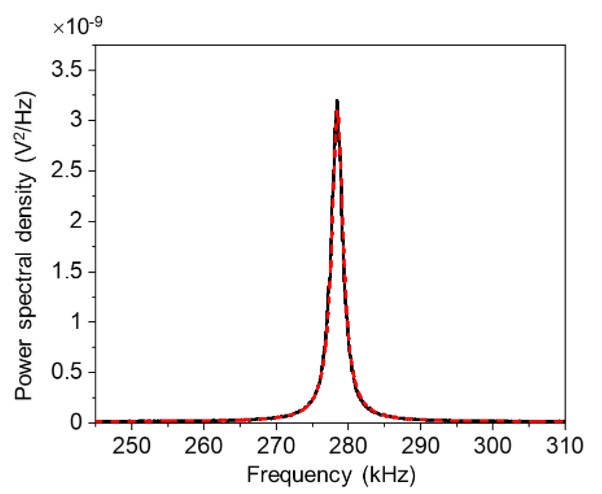
Fig. 4. Thermal noise spectrum of the cantilever used. The red dashed line presents the curve fit based on simple harmonic oscillator model.

  After normal and lateral calibrations, the LFM measurement was performed on a thin flake of graphene deposited on a silicon (Si) substrate. The normal force (setpoint), scan area, and scan rate were set to 10 nN, 2×1 µm2, and 0.5 Hz, respectively. Relatively low scan rate was used to make sure that the tip could track the surface well. The topography and LFM channels were monitored during scanning.
  LFM measurement result is summarized in Fig. 5. The height, lateral forward (FW), and lateral backward (BW) images along with the cross-sectional profiles are presented in the figure. The thickness of graphene layer estimated from the cross-sectional height profile was about 1 nm. Also, the material effect on friction force is clearly shown in the friction loop data. It was clearly observed that Si substrate exhibits higher frictional properties compared to graphene sample. In addition, it should be noted that the lateral forward and backward signals are expected to be symmetrical about the zero-horizontal axis, as shown in Fig. 1(b). However, in practical measurement, the laser spot is not always located at the zero-lateral position [(2 + 4) = (1 + 3)] initially. As a result, the entire friction loop can be shifted upward or downward along the vertical axis. To eliminate the effect of this offset on calculation result, the friction force Ff can be calculated by considering both forward and backward scan directions, using Eq. (3). By subtracting the LFM backward signal from the LFM forward signal, the effect of vertical offset in friction loop on friction force calculation result is eliminated.

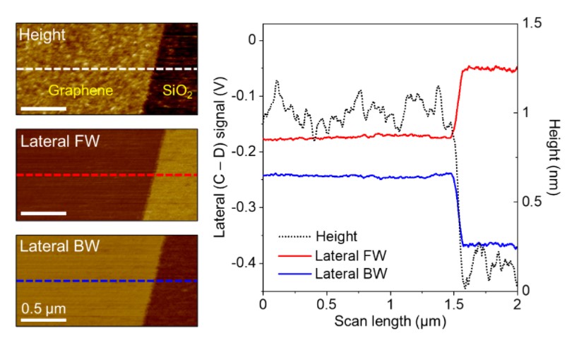
Fig. 5. Height and lateral images obtained on a thin flake of graphene deposited on Si substrate. The lateral forward and backward signals at the same scan line form a friction loop that represents the friction characteristics of sample surface.

Fig. 6 shows the friction force calculation result based on Eq. (3). Friction force was determined to be 2.9 nN and 13.7 nN when the tip slide against graphene and Si substrate, respectively. The friction force obtained on Si increases by a factor of 4.7 compared to the graphene flake. Low friction characteristics of graphene suggests it can be a potential candidate as solid lubrication layer for moving mechanical parts of micro- and nano- devices.

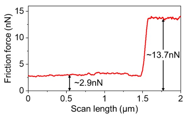
Fig. 6. Friction force calculated from the friction loop in Fig. 5. The silicon substrate exhibits higher frictional properties than the graphene sample.

  Nevertheless, there are a few criteria should be met for more accurate frictional properties measurement. In-plane spring constant of the cantilever should be large enough so that only twist of the cantilever occurs during lateral scanning [10]. To improve the accuracy of lateral force sensitivity determination based on Lateral AFM Thermal-Sader method, the cantilever geometry should meet the criterion of Sader’s method (i.e., high length-to-width ratio) [5,7]. Also, the torsional resonance of the cantilever should not exceed the bandwidth of the AFM instrument. Usually, conventional cantilevers for LFM measurement satisfy these criteria. However, for special cases (e.g., home-made cantilever, modified cantilever), it is recommended to check these criteria before measurement.

References

[1] D. Berman, A. Erdemir, A. V Sumant, Graphene: a new emerging lubricant, Mater. Today. 17 (2014) 31–42.
[1] B.-C. Tran-Khac, H.-J. Kim, F.W. DelRio, K.-H. Chung, Operational and environmental conditions regulate the frictional behavior of two-dimensional materials, Appl. Surf. Sci. 483 (2019) 34–44.
[3] Q.D. Nguyen, K.-H. Chung, Effect of tip shape on nanomechanical properties measurements using AFM, Ultramicroscopy. 202 (2019) 1–9.
[4] J.L. Hutter, J. Bechhoefer, Calibration of atomic‐force microscope tips, Rev. Sci. Instrum. 64 (1993) 1868–1873.
[5] K. Wagner, P. Cheng, D. Vezenov, Noncontact Method for Calibration of Lateral Forces in Scanning Force Microscopy, Langmuir. 27 (2011) 4635–4644.
[6] N. Mullin, J.K. Hobbs, A non-contact, thermal noise based method for the calibration of lateral deflection sensitivity in atomic force microscopy, Rev. Sci. Instrum. 85 (2014) 113703.
[7] B.C. Tran Khac, K.-H. Chung, Quantitative assessment of contact and non-contact lateral force calibration methods for atomic force microscopy, Ultramicroscopy. 161 (2016) 41–50.
[8] C.P. Green, H. Lioe, J.P. Cleveland, R. Proksch, P. Mulvaney, J.E. Sader, Normal and torsional spring constants of atomic force microscope cantilevers, Rev. Sci. Instrum. 75 (2004) 1988–1996.
[9] Online calculator is available at: http://www.ampc.ms.unimelb.edu.au/afm/calibration.html.
[10] J.E. Sader, C.P. Green, In-plane deformation of cantilever plates with applications to lateral force microscopy, Rev. Sci. Instrum. 75 (2004) 878–883.